Experiment

Setup

import matplotlib.pyplot as plt
import numpy as np
import seaborn as sns
from tqdm.auto import tqdm

from swiift import Experiment, Ocean, Ice, Floe, DiscreteSpectrum
from swiift.api.api import Step
from swiift.lib.physics import FluidSurfaceHandler

Introduction

The most straightforward way to use SWIIFT, is through the API exposed by Experiment objects.

In this example, we present the steps to initiate and run a wave fracture simulation.

Ocean and gravity waves

Experiment instances are preferentially initialised through the factory method create().

This method takes gravity, ocean and spectrum (respectively of type float, Ocean, and DiscreteSpectrum) as mandatory parameters. It correctly initialises the attribute domain, an object that handles the coupling between ocean and spectrum by determining the wavenumbers associated to the forcing frequencies. It also initialise the fracture handler, and the attribute history, that will be populated when the experiment is run.

# All the physical quantities are given in the appropriate SI unit, or
# derived unit.
# Therefore, times are expressed in seconds, lengths in metres,
# accelerations in metre per square second, energies in joules, etc.

# Set the value of gravity.
gravity = 9.8

# Set the characteristics of an `Ocean` object and instantiate it.
depth = 300
ocean = Ocean(depth=depth)

# Set the period and amplitude of the wave forcing,
# and use them to instantiate a `DiscreteSpectrum` object.
# Because we use scalar as parameters here, the model will be forced
# by a simple monochromatic wave.
period = 6
amplitude = .25
spectrum = DiscreteSpectrum(amplitude, 1 / period)

# Gravity, spectrum and ocean are combined
# to instantiate an `Experiment` object.
experiment = Experiment.create(
    gravity,
    spectrum,
    ocean,
)

# The attributes of an ``Experiment`` instance.
# The current time of the experiment; increases when the experiment is run.
# Initialised at 0 s.
print(f"Time: {experiment.time} s\n")
# The array of existing timesteps, that can index the history.
# Empty for now, has the experiment was not run.
print(f"Timesteps: {experiment.timesteps}\n")
# The history, a dictionary of ``Step`` objects associated to individual timesteps.
# Empty for now, has the experiment was not run.
print(f"History: {experiment.history}\n")
# The experiment's domain, the container that holds information on
# the fluid, the forcing, and the floes.
# It does not have any floes for now. We'll add them at the next step.
print(f"Domain: {experiment.domain}\n")
# Note the attribute ``fsw``, that combines the properties of ``ocean``
# and ``spectrum``, as well as ``gravity``, to compute wavenumbers.
print(f"`fsw` property of the domain: {experiment.domain.fsw}\n")
# The attribute ``subdomains``, for now an empty list, shows there is
# no floes in the domain.
print(f"Subdomains: {experiment.domain.subdomains}\n")
# The experiment's fracture handler.
# It determines the fracture parametrisation that will be used.
print(f"Experiment's fracture handler: {experiment.fracture_handler}")

Time: 0 s

Timesteps: []

History: {}

Domain: Domain(gravity=9.8, spectrum=DiscreteSpectrum(amplitudes=array([0.25]), frequencies=array([0.16666667]), phases=array([0.])), fsw=FreeSurfaceWaves(ocean=Ocean(depth=300, density=1025), wavenumbers=array([0.11190028])), growth_params=None)

`fsw` property of the domain: FreeSurfaceWaves(ocean=Ocean(depth=300, density=1025), wavenumbers=array([0.11190028]))

Subdomains: []

Experiment's fracture handler: BinaryFracture(coef_nd=4, scattering_handler=ContinuousScatteringHandler())

Ice and floe

A Floe can then be added to the Experiment. Floes bring together three properties: location (left_edge), extent (length), and ice characteristics (ice). The latter are grouped in an object Ice.

Once constructed, the floe (or a collection of floes) can be added to an existing Experiment with a call to the method add_floes().

# Set mechanical characteristics and instantiate an `Ice` object.
thickness = 0.5
youngs_modulus = 4e9
poissons_ratio = 0.3
ice = Ice(
    thickness=thickness,
    poissons_ratio=poissons_ratio,
    youngs_modulus=youngs_modulus,
)
# Properties like the flexural rigidity, that can be inferred from
# the initialisation parameters, are automatically computed.
print(f"Flexural rigidity: {ice.flex_rigidity:e} Pa m^3.\n")

# Set position and extent and instantiate a `Floe` object.
left_edge = 12.3
length = 236.1
floe = Floe(left_edge=left_edge, length=length, ice=ice)
# Floes are analogous to segments, bounded by two points in space.
print(f"Floe goes from x={floe.left_edge} m to x={floe.right_edge:.1f} m.\n")

# Add the floe to the experiment's domain.
experiment.add_floes(floe)

# Let us inspect attributes again.
# The time has not changed.
print(f"Time: {experiment.time} s.\n")
# However, adding a floe to the experiment added this timestep as
# a first key to the history.
print(f"Timesteps: {experiment.timesteps}.\n")
# The associated value is a ``Step`` object, that hold
# its own ``subdomains`` attribute.
print(f"History: {experiment.history}\n")
# The ``subdomains`` property of ``experiment.domain`` is identical to
# that of the last step in the history.
print(f"Subdomains: {experiment.domain.subdomains}\n")
# Subdomains are a list, that can be indexed to access
# the ``WavesUnderFloe`` objects it contains.
print(f"First subdomain: {experiment.domain.subdomains[0]}\n")
# In particular, these have an attribute ``wui``.
# Like ``domain.fsw``, these combine the forcing information with other
# quantities to determine the wavenumbers propagating under the ice.
print(
    "`wui` property of the first subdomain: "
    f"{experiment.domain.subdomains[0].wui}\n"
)
# These ``WavesUnderIce`` objects compose wavenumbers, attenuation, and
# ice, which extends the class ``Ice`` to include properties that need
# ocean and gravity to be defined, like draught and freeboard of the ice.
print(
    "`ice` property of the `wui` property of the first subdomain: "
    f"{experiment.domain.subdomains[0].wui.ice}"
)

Flexural rigidity: 4.578755e+07 Pa m^3.

Floe goes from x=12.3 m to x=248.4 m.

Time: 0 s.

Timesteps: [0].

History: {0: Step(subdomains=(WavesUnderFloe(left_edge=12.3, length=236.1, wui=WavesUnderIce(ice=FloatingIce(density=922.5, frac_toughness=100000.0, poissons_ratio=0.3, strain_threshold=3e-05, thickness=0.5, youngs_modulus=4000000000.0, draft=0.45, dud=299.55, elastic_length_pow4=4558.242487560556)), edge_amplitudes=array([0.04830009+0.24528983j]), generation=0),), growth_params=None)}

Subdomains: [WavesUnderFloe(left_edge=12.3, length=236.1, wui=WavesUnderIce(ice=FloatingIce(density=922.5, frac_toughness=100000.0, poissons_ratio=0.3, strain_threshold=3e-05, thickness=0.5, youngs_modulus=4000000000.0, draft=0.45, dud=299.55, elastic_length_pow4=4558.242487560556)), edge_amplitudes=array([0.04830009+0.24528983j]), generation=0)]

First subdomain: WavesUnderFloe(left_edge=12.3, length=236.1, wui=WavesUnderIce(ice=FloatingIce(density=922.5, frac_toughness=100000.0, poissons_ratio=0.3, strain_threshold=3e-05, thickness=0.5, youngs_modulus=4000000000.0, draft=0.45, dud=299.55, elastic_length_pow4=4558.242487560556)), edge_amplitudes=array([0.04830009+0.24528983j]), generation=0)

`wui` property of the first subdomain: WavesUnderIce(ice=FloatingIce(density=922.5, frac_toughness=100000.0, poissons_ratio=0.3, strain_threshold=3e-05, thickness=0.5, youngs_modulus=4000000000.0, draft=0.45, dud=299.55, elastic_length_pow4=4558.242487560556))

`ice` property of the `wui` property of the first subdomain: FloatingIce(density=922.5, frac_toughness=100000.0, poissons_ratio=0.3, strain_threshold=3e-05, thickness=0.5, youngs_modulus=4000000000.0, draft=0.45, dud=299.55, elastic_length_pow4=4558.242487560556)

Run the experiment

Single step

An experiment is moved forward in time by calling the method step(). It takes a time increment as mandatory parameter.

Warning

This method modifies the instance in-place. The wave is advected across the domain, the time attribute of the instance is incremented, and its history updated.

# We extract the first (and for now, only) subdomain to access its
# attributes more easily.
wuf = experiment.domain.subdomains[0]
# We establish in Mokus et al. (2026) a lower bound and an upper bound
# on the timestep.
# The former comes from fracture theory and represents the time
# necessary for a fracture to propagate entirely through the thickness;
# the second is empirical and was selected to ensure convergence in a
# repeated fracture experiment.
shear_wave_speed = np.sqrt(ice.youngs_modulus / (2 * ice.density * (1 + ice.poissons_ratio)))
print(f"{shear_wave_speed} m s^-1")
min_time = ice.thickness / shear_wave_speed
print(f"{min_time} s")
phase_speed = (spectrum.angular_frequencies / wuf.wui.wavenumbers).squeeze()
print(f"{phase_speed} m s^-1")
security_factor = 1 / 5
max_time = security_factor * spectrum.amplitudes.squeeze() / phase_speed
print(f"{max_time} s")
print(f"Time ratio: {max_time / min_time}")  # Greater than 1, good news!

# We can now select the larger time as our simulation timestep.
timestep = max_time
experiment.step(timestep)

1291.3980737100994 m s^-1
0.0003871772849742092 s
11.661232222403259 m s^-1
0.004287711542519605 s
Time ratio: 11.074284853268754

# Let us inspect attributes again.
# This time, the time has changed, increased by ``timestep``.
print(f"Time: {experiment.time} s.\n")
# This new time was added to the history.
print(f"Timesteps: {experiment.timesteps} s.\n")
print(f"Length of history: {len(experiment.history)}")
# The final state of the experiment (corresponding to the current value
# of its attribute ``time`` is accessed with the convenience method
# ``get_final_state``.
print(f"Number of floes: {len(experiment.get_final_state().subdomains)}")
print(
    "Length of floes: "
    f"{np.asarray([_w.length for _w in experiment.get_final_state().subdomains])} m."
)
# Fractures conserve ice area (that is, in our 1D case, ice length).
is_length_the_same = np.isclose(
    sum([_w.length for _w in experiment.get_final_state().subdomains]),
    floe.length,
)
print(
    "Total ice length after fracture is the same as before: "
    f"{is_length_the_same}\n"
)
# The wave has been advected.
# We can confirm it by looking at the wave phase at the edge of the first (leftmost) floe.
phase_0 = np.angle(experiment.history[0].subdomains[0].edge_amplitudes).squeeze()
phase_t = np.angle(experiment.get_final_state().subdomains[0].edge_amplitudes).squeeze()
print(
    f"Wave phase at x={floe.left_edge} m, t=0 s: "
    f"{phase_0} rad"
)
print(
    f"Wave phase at x={floe.left_edge} m, t={experiment.time} s: "
    f"{phase_t} rad"
)
print(
    "Difference in phases: "
    f"{phase_t - phase_0} rad."
)
print(
    r"Timestep × angular frequency: "
    f"{timestep * spectrum.angular_frequencies.squeeze()} rad."
)

Time: 0.004287711542519605 s.

Timesteps: [0.         0.00428771] s.

Length of history: 2
Number of floes: 2
Length of floes: [ 34.35425515 201.74574485] m.
Total ice length after fracture is the same as before: True

Wave phase at x=12.3 m, t=0 s: 1.3763734028730055 rad
Wave phase at x=12.3 m, t=0.004287711542519605 s: 1.3718833218454416 rad
Difference in phases: -0.004490081027563875 rad.
Timestep × angular frequency: 0.004490081027563917 rad.

Multiple steps

The experiment can also be run for a specified number of steps by calling the method run() method. The total time, as well as the duration of a timestep, must be specified.

Warning

This method also modifies the instance in-place, by repeatedly calling step().

# Let's run the experiment for one extra second.
total_time = 3
# We instantiate a progress bar for convenient tracking.
n_steps = int(np.ceil(total_time / timestep).astype(int))
print(f"Number of timesteps to run: {n_steps}")
pbar = tqdm(total=n_steps)
experiment.run(
    total_time,
    timestep,
    verbose=2,  # Tell the program to write to stdout on fractures
    pbar=pbar,
    dump_final=False,  # To keep the history in memory
    
)

Number of timesteps to run: 700

t = 0.009 s; N_f = 4

t = 0.013 s; N_f = 6

t = 0.017 s; N_f = 10
t = 0.021 s; N_f = 14

t = 0.026 s; N_f = 16
t = 0.030 s; N_f = 18

t = 0.141 s; N_f = 19

t = 0.172 s; N_f = 20

t = 0.596 s; N_f = 21

t = 1.972 s; N_f = 22

# Let us inspect attributes again.
print(f"Time: {experiment.time} s.")
print(f"Length of history: {len(experiment.history)}.")
# The final state of the experiment (corresponding to the current value
# of its attribute ``time`` is accessed with the convenience method
# ``get_final_state``.
print(f"Number of floes: {len(experiment.get_final_state().subdomains)}")
print(
    "Length of floes: "
    f"{np.asarray([_w.length for _w in experiment.get_final_state().subdomains])} m."
)
# Fractures conserve ice area (that is, in our 1D case, ice length).
is_length_the_same = np.isclose(
    sum([_w.length for _w in experiment.get_final_state().subdomains]),
    floe.length,
)
print(
    "Total ice length after fracture is the same as before: "
    f"{is_length_the_same}\n"
)

Time: 3.0056857913062482 s.
Length of history: 702.
Number of floes: 22
Length of floes: [ 5.64177269 13.52769477 15.18478769  8.61617131  9.74803598 11.13716787
  8.87792195  8.4394007   8.80910952 16.92499919 14.97156451  8.61539743
  8.73203258  6.33835087 13.55364126 15.51786234  8.67925219  9.92593494
 10.94690929  8.88487497  8.63859646 14.3885215 ] m.
Total ice length after fracture is the same as before: True

Plotting some results

import matplotlib as mpl

def floe_state_gen(
    xx: np.ndarray, tt: np.ndarray, _exp: Experiment, post_f_times: np.ndarray
) -> np.ndarray:
    """Generate mesh data to plot from floe generation.

    Paramters
    ---------
    xx : np.ndarray
        1D array of boundaries between floes.
    tt : np.ndarray
        1D array of timesteps.
    _exp : Experiment
        Experiment object to build a mesh for.
    post_f_times : np.ndarray
        1D array of times following fractures.

    Returns
    -------
    np.ndarray
        2D array of type int containing the generation mesh associated
        with the parameters.
        
    """
    # Initialise a mesh of integers with -1 as sentinel value.
    # Rows are time and columns space.
    floe_state = np.full((len(tt) - 1, len(xx) - 1), -1, dtype=int)
    # The first timestep has only a single floe of generation 1.
    floe_state[0, :] = 0

    # Iterating on the timesteps following fracture, gradually build
    # the mesh by recovering spatial (left edge, length) and generation
    # information for each floe (inner loop) at each step (outer loop).
    for i, _t in enumerate(post_f_times, start=1):
        le, lgt, gen = get_edges_lengths_gen(_exp.history[_t])
        for _le, _l, _gen in zip(le, lgt, gen):
            # A floe goes from left edge (included) to right edge (excluded).
            mask = (xx >= _le) & (xx < _le + _l)
            floe_state[i, mask[:-1]] = _gen
    # Check that every cell in the mesh has had a value attributed.
    assert np.all(floe_state > -1)
    return floe_state


def get_edges_lengths_gen(step: Step):
    """Get edge, length, and generation of each floe in a step.

    Paramters
    ---------
    step : Step
        The step to work on.
        
    """
    # `Step` objects are simple namedtuple objects representing
    # the geometry in the model at a given timestep.
    # The important field now is `subdomains`, the list of floe
    # objects in the domain.
    subdomains = step.subdomains
    # Sequentially recover, then return, the left edge,
    # length, and generation, of each floe in the domain.
    edges, lengths, generations = zip(*(
        (_w.left_edge, _w.length, _w.generation) for _w in subdomains
    ))
    return np.vstack((edges, lengths, generations))


def make_gen_pmesh(_exp: Experiment):
    """Generate and display a space-time plot of generations.

    Parameters
    ----------
    _exp : Experiment
        The experiment to generate the figure of.
        
    """
    # Build an array of times.
    # The first time is the first key in `history`, the last time
    # is the Experiment's current `time` attribute.
    first_time, final_time = next(iter(_exp.history)), _exp.time
    # This convenience method returns all the times (keys in `history`)
    # immediately following breakups.
    post_f_times = _exp.get_post_fracture_times()
    # Extend the post-breakup times with our initial and final times.
    extended_post_times = np.hstack((first_time, post_f_times, final_time))

    # Build an array of x coordinates.
    # Recover the final state, identify the left edge of each floe,
    # and add the right edge of the rightmost floe to close the domain.
    final_state = _exp.get_final_state()
    xx, tt = (
        np.hstack((
            get_edges_lengths_gen(final_state)[0],
            final_state.subdomains[-1].right_edge,
        )),
        extended_post_times,
    )

    # Get the mesh values0
    floe_state = floe_state_gen(xx, tt, _exp, post_f_times)

    # Prep a discrete colourbar.
    generations = np.unique(floe_state)
    # If N categories, we need N+1 bounds.
    bounds = np.arange(len(generations) + 1)
    # Artifical 0.5 offset for label centring.
    _bounds = bounds - .5
    norm = mpl.colors.BoundaryNorm(_bounds, len(generations))
    fmt = mpl.ticker.FuncFormatter(lambda x, pos: generations[norm(x)])
    cmap = mpl.colors.LinearSegmentedColormap.from_list(
        "name",
        mpl.colormaps.get_cmap("grey")(generations / generations.max()), len(generations)
    )
    # Plot, add label decoration, show and close.
    plt.pcolormesh(xx, tt, floe_state, cmap=cmap, norm=norm)    
    plt.colorbar(ticks=generations, format=fmt, label="Floe generation")
    plt.xlabel("$x$ (m)")
    plt.ylabel("$t$ (s)")
    plt.show()
    plt.close()

Space-time floe generations

from swiift.model.model import WavesUnderFloe

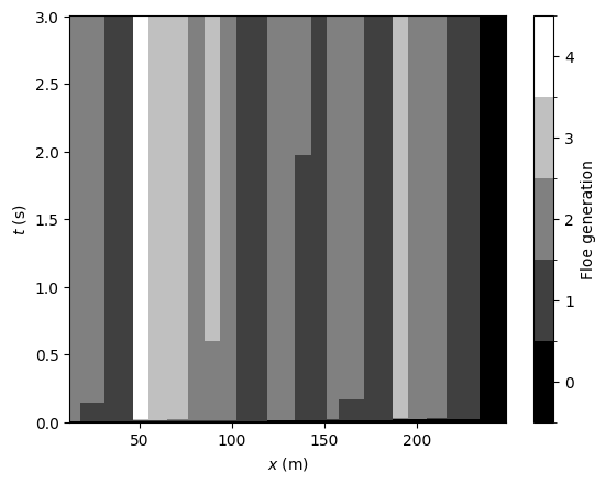
Fractured floes have an attribute generation that keeps track of the number of fracture events having led to them. Floes manually added to the domain have their generation set to 0. When a fracture occurs, the right fragment keeps the generation of the parent floe, and the left fragment has its generation incremented by 1.

The next cell shows the space-time evolution of the floes generation during the experiment. Feel free to inspect the code of the function that builds the figure, to get some insight on swiift innards.

make_gen_pmesh(experiment)

Final FSD

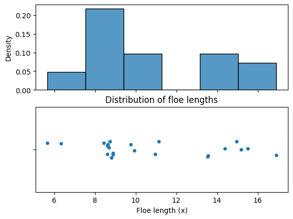
An important quantity is the floe size distribution after repeated breakup. It can easily be constructed and visualise as demonstrated below.

The method get_final_state() conveniently gives access to the last Step of the simulation: calling experiment.get_final_state() is equivalent to calling experiment.history[experiment.time]. This Step object is simply a namedtuple; for our purpose, the important field is subdomains. A subdomain is simply a Floe-derived object, that contains length information.

# Get the final subdomains.
final_subdomains = experiment.get_final_state().subdomains
# For every subdomain, recover its length.
floe_lengths = np.asarray([_w.length for _w in final_subdomains])

fig, axes = plt.subplots(2, sharex=True)

# Plot the density as a histogram.
sns.histplot(floe_lengths, stat="density", ax=axes[0])
# Alternatively, plot the density as a stripplot, more legible when
# observations are few.
# Each dot represents an observation, the y-axis is only here to
# prevent the dots from overlapping.
sns.stripplot(x=floe_lengths, ax=axes[1])

plt.xlabel("Floe length (x)")
plt.title("Distribution of floe lengths")
plt.show()
plt.close()

Number of floes in time

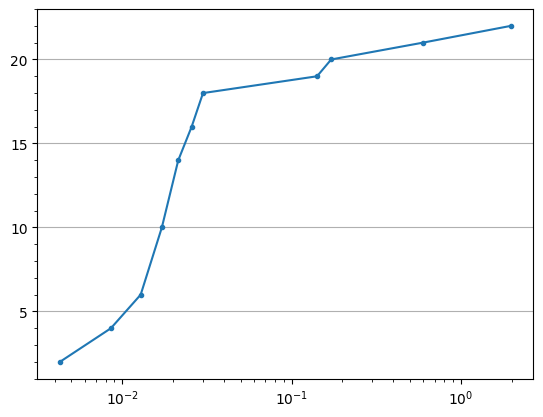
One might also be interested in the time-dependent evolution of the number of floes.

# Get the time following fracture events.
post_f_times = experiment.get_post_fracture_times()
# For each of these times, recover the length of the domain.
n_floes = [len(experiment.history[_pf_time].subdomains) for _pf_time in post_f_times]

plt.plot(post_f_times, n_floes, ".-")
# Number of floes grows fast for a few timesteps then slows down.
plt.xscale("log")
# We're plotting integers, so avoid floating point ticks.
# Add a nice grid.
plt.gca().yaxis.set_major_locator(plt.MultipleLocator(5))
plt.gca().yaxis.set_minor_locator(plt.MultipleLocator(1))
plt.grid(axis="y")
plt.show()
plt.close()

Spatial evolution

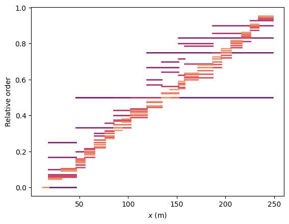
The domain is iteratively populated with new floes. The way these are spatially aranged, that is, which floe breaks and when, can be visualised as illustrated below.

# Instantiate a perceptually uniform colour palette with enough colours.
palette = sns.color_palette("flare_r", n_colors=len(post_f_times))

with palette:
    for _it, _t in enumerate(post_f_times):
        _s = experiment.history[_t]
        # Construct a step function to illustrate the time evolution
        # of the spatial arrangement of the domain.
        # At each (post-fracture) timestep, we get the boundaries of
        # each floe.
        # We use these to draw a segment.
        # The next segment is then drawn a little higher, in a step pattern.
        # The y-axis is thus the floe rank number within the array,
        # normalised by the size of the array.
        # The luminance increases at each timestep: "more recent" times
        # are lighter in colour.
        for i, _w in enumerate(_s.subdomains):
            plt.plot(
                [_w.left_edge, _w.right_edge],
                [i / len(_s.subdomains)]*2,
                f"C{_it}",
                lw=2,
            )
    plt.xlabel("$x$ (m)")
    plt.ylabel("Relative order")
    plt.show()
    plt.close()

# Same thing using maplotlib builtin `plt.stairs`, which adds vertical
# connecting lines between horizontal segments.
# with palette:
#     for _it, _t in enumerate(experiment.get_post_fracture_times()):
#         _s = experiment.history[_t].subdomains
#         edges = np.asarray([_w.left_edge for _w in _s] + [_s[-1].right_edge])
#         values = np.arange(len(edges) - 1) / (len(edges) - 2)
#         plt.stairs(
#             values,
#             edges,
#             edgecolor=f"C{_it}",
#             lw=2,
#         )
#     plt.show()
#     plt.close()